Create a PivotTable to analyze worksheet data
A PivotTable is a powerful tool to calculate, summarize, and analyze data that lets you see comparisons, patterns, and trends in your data.
PivotTables work a little bit differently depending on what platform you are using to run Excel.

Create a PivotTable in Excel for Windows
-
Select the cells you want to create a PivotTable from.
Note: Your data shouldn't have any empty rows or columns. It must have only a single-row heading.
-
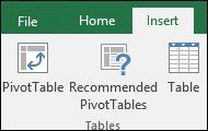
Select Insert > PivotTable.
-
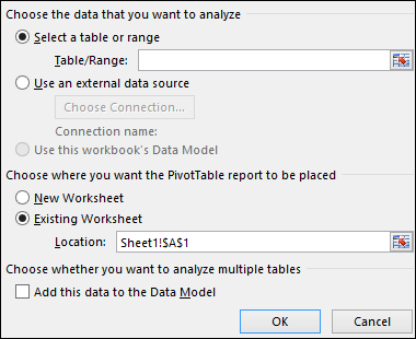
Under Choose the data that you want to analyze, select Select a table or range.
-
In Table/Range, verify the cell range.
-
Under Choose where you want the PivotTable report to be placed, select New worksheet to place the PivotTable in a new worksheet or Existing worksheet and then select the location you want the PivotTable to appear.
-
Select OK.
Building out your PivotTable
-
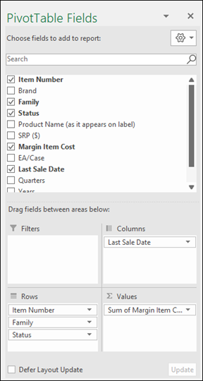
To add a field to your PivotTable, select the field name checkbox in the PivotTables Fields pane.
Note: Selected fields are added to their default areas: non-numeric fields are added to Rows, date and time hierarchies are added to Columns, and numeric fields are added to Values.
-
To move a field from one area to another, drag the field to the target area.