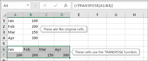
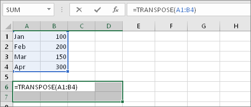
Sometimes you need to switch or rotate cells. You can do this by copying, pasting, and using the Transpose option. But doing that creates duplicated data. If you don't want that, you can type a formula instead using the TRANSPOSE function. For example, in the following picture the formula =TRANSPOSE(A1:B4) takes the cells A1 through B4 and arranges them horizontally.
Note: If you have a current version of Microsoft 365 , then you can input the formula in the top-left-cell of the output range, then press ENTER to confirm the formula as a dynamic array formula. Otherwise, the formula must be entered as a legacy array formula by first selecting the output range, input the formula in the top-left-cell of the output range, then press Ctrl+Shift+Enter to confirm it. Excel inserts curly brackets at the beginning and end of the formula for you. For more information on array formulas, see Guidelines and examples of array formulas.
First select some blank cells. But make sure to select the same number of cells as the original set of cells, but in the other direction. For example, there are 8 cells here that are arranged vertically:

So, we need to select eight horizontal cells, like this:

This is where the new, transposed cells will end up.
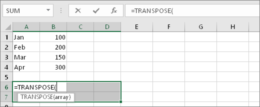
With those blank cells still selected, type: =TRANSPOSE(
Excel will look similar to this:
Notice that the eight cells are still selected even though we have started typing a formula.
Now type the range of the cells you want to transpose. In this example, we want to transpose cells from A1 to B4. So the formula for this example would be: =TRANSPOSE(A1:B4) -- but don't press ENTER yet! Just stop typing, and go to the next step.
Excel will look similar to this:
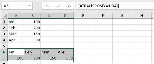
Now press CTRL+SHIFT+ENTER. Why? Because the TRANSPOSE function is only used in array formulas, and that's how you finish an array formula. An array formula, in short, is a formula that gets applied to more than one cell. Because you selected more than one cell in step 1 (you did, didn't you?), the formula will get applied to more than one cell. Here's the result after pressing CTRL+SHIFT+ENTER:
You don't have to type the range by hand. After typing =TRANSPOSE( you can use your mouse to select the range. Just click and drag from the beginning of the range to the end. But remember: press CTRL+SHIFT+ENTER when you are done, not ENTER by itself.
The TRANSPOSE function returns a vertical range of cells as a horizontal range, or vice versa. The TRANSPOSE function must be entered as an array formula in a range that has the same number of rows and columns, respectively, as the source range has columns and rows. Use TRANSPOSE to shift the vertical and horizontal orientation of an array or range on a worksheet.
TRANSPOSE(array)
The TRANSPOSE function syntax has the following argument:
array Required. An array or range of cells on a worksheet that you want to transpose. The transpose of an array is created by using the first row of the array as the first column of the new array, the second row of the array as the second column of the new array, and so on. If you're not sure of how to enter an array formula, see Create an array formula.